Update to this. UK government have finally put this out. Finally some decent stats!
Also, here's the mobile version, but the other one is better.

Update to this. UK government have finally put this out. Finally some decent stats!
Also, here's the mobile version, but the other one is better.
After reading through my coronavirus post, my friend Joe had stated that I should have had more flow diagrams in it.
So Joe, this diagram is especially for you:
So this virus outbreak thing is interesting isn't it?
As a mathematician-in-training, what I'm finding more interesting is the lack of good statistics on what's happening. The UK government were initially publishing new infections within England and in the whole of the UK. In addition, they were publishing the total UK infected, and total UK deaths. They stopped reporting anything on March 5th.
Though as well as keeping track of government announcements, I've also been keeping record of daily updates that the World Health Organisation (WHO) have been making.
Here's a link to their European map.
Here's a link to their global map.
On a daily basis, I've been recording UK totals from their site. You can see them graphed below:
You can't see it, but the values for the first 9 days are just two people.
Though see how there's a dip on March 16th? How could there possibly be a dip in cases for one day by over 100 people? It seems even the pros can get their numbers wrong. Bad work, WHO. 🙁
Also, you'll notice from around March 5th to March 8th, it goes flat. These are days on which I didn't check the figures.
From these total cases per day, I've calculated new cases per day.
See that negative number of new cases on March 16th? Insert eyeroll emoji.
There's also a spike on March 9th, this is just total new cases from March 5th to March 9th. -catching up from when I didn't check on the totals on these days.
But as you can see, as predicted, this initial growth is basically exponential. Fairly typical for an epidemic apparently.
So the big question is... what next?! -and here's where my mathematics and statistics study comes in handy... I've recently finished a section on epidemics! What better time to apply some of my learning!
First off, it's worth mentioning that all the epidemic modelling I've learned about assumes homogeneous mixing. This is the kind of mixing that occurs in a family home. ie: there's more or less an equal chance of me having contact with one person than there is anyone else. In real life this, of course, isn't true. Living in London, I'm less likely to be in contact with someone in Edinburgh than I am someone I travel with on the London Underground every day. Also important point: homogeneous mixing means no quarantining. So all of the below is essentially average worst-case.
So with the proviso that these results will probably (more than likely) be wildly inaccurate, let's get started! We need a few important numbers, some of which we've already got:

Where:
Which is fine, but how do we know what γ and β are? Well there's a number called R0 ("R-naught") that I've NOT been taught about that represents the contagiousness of a virus. Interestingly, I've found two completely opposed descriptions of this number:
Though we all know how reliable wikipedia is, and I've just found this Stanford paper which supports the towardsdatascience description:

Therefore:

Hooray. Imperial College London seems to estimate the R0 of COVID-19 to be 2.4, so let's run with that.

Once we have all this, we can work out the maximum number of infectives at any one time. ie: the peak of the infection in the population, ymax:

Now we can plug all the numbers in to find ymax! So:

Hence:

Which is 42.5% of the population infected at one time! Ouch! At least you'll know that if we (in our theoretical UK) hit 28 million with no quarantining, we'd be at the peak of the outbreak.
Other sources state that COVID-19 actually has a range of R0 values, 1.4-3.8-ish, so the band of possible outcomes without quarantining is actually quite broad. But from this it's possible to work out a best-case/worse-case comparison:
An R0 of 1.4 would mean a max of 12.2 million (18% of the population), and an R0 of 3.8 would mean a max of 39.4 million (58% of the population) at one time.
The following assumes that the whole debacle is over. Everyone that has caught the virus from it has now recovered. How many people were not affected?
This is found using the following iteration formula:

Initially x_{inf,j} is zero, and you use your result x_{inf,j+1} to calculate x_{inf,j+2}, and so on. This eventually settles down to the number of people not affected!
So using the power of spreadsheets, and not taking up the space here with columns and columns of numbers:
You can imagine that an increase in quarantining means a lower R0. Seems that could have a big effect.
#ImNotAStatisticianButItsStillFunLookingAtNumbers
Two thirds of the way through my assignments!
Again, fairly happy with the mark I received for this, but there were some aspects of this assignment I found challenging, and some where I thought I might've done quite well on, but slipped up in some way.
Let's cover some areas here:
For these questions I had to find a real-world process that could be modelled with the given mathematical objects/processes. Kind of the opposite of a mathematical modelling problem.
I found these tasks really difficult. What I found to be the worst aspect about getting this kind of question wrong is that it's not necessarily my understanding of the mathematical process that's flawed. I feel in each of these cases, I did my best to find a real world example, knowing that the example I gave, itself, was slightly flawed. So despite the fact that I can perfectly explain each mathematical process, I couldn't explain how each could be applied to a real world process so lost marks.
The two models were the Galton-Watson branching process, and the simple random walk (specifically, a particle executing a simple random walk on the line with two absorbing barriers).
The two typical examples that are referred to in my texts are genetics and mutations for the Galton-Watson branching process:
"A mutation is a spontaneous transformation of a particular gene into a different form, and this can occur by chance at any time... The mutant gene becomes the ancestor of a branching process, and geneticists are particularly interested in the probability that the mutation will eventually die out."
For the simple random walk, the example of the "gambler's ruin" was given. Imagine two people with £10 each, each of them betting on an event. If one of the two loses the bet, they give £1 to the other (the random walk on the line). If one of them runs out of money, then they lose (one of the "absorbing barriers" are hit).
In coming up with answers, I could've used Google, but that would've been cheating. However, now I've completed the assignment and received my grade, Google is my best friend in finding suitable answers here...
Seems you can use the Galton-Watson branching process to determine the extinction of a family name, and I found a good example of a random walk with absorbing barriers in this MIT paper, featuring a little flea called Stencil. It discusses the probability of him falling over the Cliff of Doom in front of him, or the Pit of Disaster behind him.
A couple of my answers here and there were classed as being incomplete. Generalising each case:
1)
Upon finding that an answer resembles a certain construction (a probability distribution function, cumulative distribution function or generating function), as well as saying which distribution the function belongs to, you should also explicitly state the variables that appear in it. Even to anyone non-mathematical, it would be obvious to see that the variables in the general case are associated with the specific answer you arrived at. Though for assignments (and exams, presumably) this is not enough. If a general function has variables explicitly state what each one is in your answer.
eg: the p.g.f. of the modified geometric distribution is

If your answer resembles this, say what a, b, c and d are.
In addition, if your answer is a probability (or set thereof), include a statement describing them.
Note that one whole mark can be deducted for an insufficient conclusion (apparently).
2)
Don't forget your definitions.
Specifically:
To calculate the variance of the position of a particle (along the random walk line) after n steps, you can just sum the variances of each step. However this only works because each individual step is independent of the last (one of the properties of the random walk). Due to the fact that I didn't mention this definition of the variance of a particle in a random walk, I lost half a mark. Not massive, but where you can mention a definition, mention it.
I struggled with this, and although I arrived at the correct answer, the method I had used was entirely wrong (and also a little inelegant).
In this question, I covered all routes separately and so had a small handful of different probability calculations. Though when considering potential routes in a Markov chain, you can consider all routes simultaneously by taking advantage of something called an absolute probability (of the Markov chain being in a particular state at a particular time), given an initial distribution. (for my own reference this is covered in Book3, Subsection 11.2, p.87. And the handbook, p.23 item 17).
Does it matter if an arbitrary constant is positive or negative? (my ref: Q6a). I previously thought not. In this instance my constant in an integral calculation absorbed the negative sign that was in front if it. After all, a negative general constant is still a general constant, right? Well I lost half a mark here because of the absorption, and it's not currently clear why. I've asked my tutor, and I'll update it on here once I hear back from him.
Very happy with the high mark I achieved for this first assignment. Though as usual, there's a decent about to be improving. Let's start by looking at some of the more major things my tutor pointed out.
First thing is variance. How do you calculate it? Well it turns out there are a couple of ways. I just decided to use the most cumbersome way...
Calculating the mean  (expectation
  ) is easy. Multiply each number with its probability and sum them all:

The variance can then be calculated in one of two different ways:
![\sigma^{2}=E[(X-\mu)^{2}]=\sum (x-\mu)^{2}\: p(x)](http://adrianbell.me/wp-content/ql-cache/quicklatex.com-35571b9bd7cd526283e89efd65febf93_l3.png "Rendered by QuickLaTeX.com")
or

When they're written out like this, it's fairly obvious to see which method is more like the method used to calculate the mean and as such would be far less hassle. ( is an integer and
  and can be reals/rationals).
This was the question in which I lost the most marks:
Customers arrive at a shoe shop according to a Poisson process with a rate of 20 per hour.
15% of customers buy men's shoes.
60% buy women's shoes.
25% buy children's shoes.
Calculate the probability that exactly eight customers arrive in half an hour, exactly three of whom wish to purchase children's shoes.
This is such a typical mistake for me to make in statistics. I'm sure I've made this kind of mistake before...
What I ended up doing was working out the probability of the number of customers being 8 using the Poisson distribution's probability function. This was fine.
Then I used the same probability function to find the probability of 3 people wanting to buy children's shoes and multiplied them together. Wrong. At this point I needed to find the conditional probability that of the 8 customers, 3 bought children's shoes. Hence, here I shouldn't have used the Poisson distribution, I should've used the Binomial distribution instead. ie: from 8, choose 25%.
Reflecting back on the question, the correct answer seems slightly more obvious now. Especially given the "...exactly three of whom..." part of the question. I struggle to be mindful of stuff like this in the moment of answering a stats question. I suppose this part of the "translating English into maths" issue comes with more practise...
Again, my issue here was to not observe subtleties in the question. Given information about the associated distributions, I was initially meant to calculate the mean and variance of the total number of books bought in 9 hours. I managed to get this first part right, but the second part of the question asked me to calculate the index of dispersion for "this process". It turns out that "this process" refers to the process in the main question generally and not the process of books being bought within 9 hours. In this instance, ignoring the total number of books bought in 9 hours (kind of) simplifies the answer too.
In this first assignment, I lost a half a mark here and there for incorrect arithmetic. (GASP!). Upon completing my draft submission, instead of just reading through it, I should sit down and verify all my working. It will take more time, but if it scrapes 2 marks back, it could be worth it.
Other issue that occurred more than once was a lack of units when talking about rates of things happening. So there's a requirement to state " per hour" instead of just "".
Now, looking at the other integral from Oct 13th...

In my opinion, this was scarier than the first, but looking at it again, what makes it scary is the various powers. e to the power of x to the power of 2 and such.
But why should this be scary? There's practically only one tool that one could use to solve this: the only tool that includes functions of functions, integration by substitution:

In our case, the inner function:

so:

and the outer function:

Plugging all these into our "integration by substitution" tool gives:

But this is slightly different to the original integral due to that minus sign. Of course this is trivial to deal with as:

Great! So now we have the structure we require to apply integration by substitution! We can substitute all of that with  , and all the scary bits go away. So:


![=-[ e^{u}]^{u}_{0}](http://adrianbell.me/wp-content/ql-cache/quicklatex.com-fdee1a31f6da7fa7617ec9f3e6f9ab69_l3.png "Rendered by QuickLaTeX.com")


Then substituting  (=
(= ) back in:

So looking at the first one from a few days ago (Oct 13th):

I was totally lost with this. But running through some old tricks made this seem a lot more approachable. First off, moving the constant out brings a bit more clarity to the integrand,

But given the  and the exponential, we'll also probably need to use integration by parts:
![\int^{b}_{a} f(x)g^{\prime}(x)dx=[f(x)g(x)]^{b}_{a}-\int^{b}_{a} f^{\prime}(x)g(x)dx](http://adrianbell.me/wp-content/ql-cache/quicklatex.com-e698b908ecdc1b841379fbd0c0d1a7f0_l3.png "Rendered by QuickLaTeX.com")
So, as above, letting:

 ,
,
we have:


Then plugging  ,
,  ,
,  and
and  into our lovely integration by parts tool above gives:

![=\lambda\left(\left[-x^{2}\: \frac{1}{\lambda}\:e^{-\lambda x}\right]^{\infty}_{0}-\int^{\infty}_{0}-2x\:\frac{1}{\lambda}\: e^{-\lambda x}\:dx\right)](http://adrianbell.me/wp-content/ql-cache/quicklatex.com-72f718d93a8feb57f17f8a0760e4dc6c_l3.png "Rendered by QuickLaTeX.com")


Which looks very familiar with what we've started with, except is now just ! If we can reduce by another power, we'll end up with just  which will surely give us a much easier integral to solve.
So applying integration by parts again, but letting:

,
we have:

Then:

![=2\left(\left[-x\: \frac{1}{\lambda}\:e^{-\lambda x}\right]^{\infty}_{0}-\int^{\infty}_{0}-\frac{1}{\lambda}\: e^{-\lambda x}\:dx\right)](http://adrianbell.me/wp-content/ql-cache/quicklatex.com-c870494b2105ad9e7dc80450651c5ce0_l3.png "Rendered by QuickLaTeX.com")


![=\frac{2}{\lambda}\left[-\frac{1}{\lambda}\:e^{-\lambda x}\right]^{\infty}_{0}](http://adrianbell.me/wp-content/ql-cache/quicklatex.com-7cb890a455a714918d0dd3bc122a092a_l3.png "Rendered by QuickLaTeX.com")


A quick look at the mind map I produced for the whole of Book 1, very much a foundation for the rest of the materials on the module.
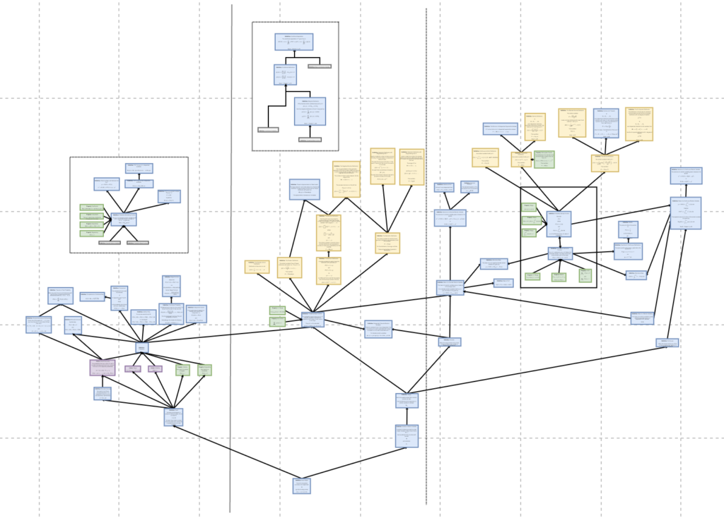
The complexity has increased necessarily, but I'd like to think the clutter has been reduced to a minimum. I was rearranging nodes as I was adding them in the hope of reducing clutter. You'll notice there are two white floating boxes not connected to anything externally. This was just to avoid clutter.
Some things to note about it that help me refer back to it:
It's split roughly into thirds, vertically. Each third is more or less a sub topic. More like themes, perhaps. Far left is foundational principles. Middle relates to basics of distributions. Far right is concepts surrounding the C.D.F. and P.D.F. (the definitions of which are in the white box in the middle of the far-right section).
Colouring helps a lot when needing to refer back to it, I found. Axioms are pink, properties are green, and definitions are blue. I found that in referring back to it, I needed some kind of differentiation between the definition of a certain distribution, and a normal definition. So all the yellow nodes you see are definitions of distributions.
In summary, to assist my understanding, I now have a graph that leads me from the most basics concept (like what an "event" is), to the definition of the standard normal distribution. I'll be referring back to this as I go!
I've just joined the Royal Statistical Society!
Putting these in a safe place for later. Found these to be a really good revision questions for integration.

and
For context, the first one formed part of a question that required me to find the variance of a random variable, and the second one involved having to find the c.d.f. from a p.d.f.
(for my own reference, this was Book 1, Activity 5.2, p. 54 and Activity 6.1, p.62)